


Horizon Robotics is a Chinese technology company that develops artificial intelligence (AI) chips used in self-driving cars and advanced driver assistance systems. We have partnered with 40+ original equipment manufacturers (OEMs) and brands globally and are the trusted choice for smart driving mass production among China's top 10 OEMs.
Architecture is shaped by scale. At the exabyte level, with hundreds of billions of files, hundreds of thousands of clients, and 200 PB of data added and deleted every week, the assumptions built into open source file systems begin to break down.
We use both JuiceFS Community Edition and Enterprise Edition to manage EB-scale data for our AIDI intelligent driving R&D platform. This article focuses on our experience with JuiceFS Community Edition, sharing how our team addressed four engineering challenges, the results we achieved, and the trade-offs we made.
New storage challenges at EB scale
AIDI supports our closed-loop intelligent driving R&D workflow. Data collected from road tests and production vehicles is filtered and labeled before entering model training. Trained models are evaluated and released, and data from newly identified issues feeds back into the pipeline. Storage underpins this entire workflow. How quickly data becomes available at each stage directly affects whether computing resources sit idle.
Over the past few years, the scale of this workflow has grown dramatically. Data capacity has increased from petabytes (PB) to exabytes (EB), while training capacity has grown from thousands to tens of thousands of GPUs. As models iterate faster and data flows back into the pipeline more frequently, storage workloads have increasingly exceeded the assumptions behind the original architecture.
Today, the platform faces the following scale and workload characteristics:
- Capacity: EB scale (1018 bytes) and still growing, well beyond the scale covered by conventional JuiceFS Community Edition testing.
- File count: Hundreds of billions (1011) of files. Individual directories, such as the trash, can contain tens of billions of entries.
- Weekly data changes: Approximately 200 PB of data added and another 200 PB deleted, leaving tens of billions of objects to be deleted from object storage.
- Client count: Hundreds of thousands of clients connecting through Kubernetes (K8s) training clusters, the Container Storage Interface (CSI), an S3-compatible gateway, and direct access through software development kits (SDKs).
- Workload characteristics: Large sequential I/O for datasets coexists with small random I/O for training checkpoints. Access frequencies vary greatly between hot and cold data, and multiple tenants share a single metadata cluster.
These conditions led us to four engineering challenges:
- How can we prevent metadata hotspots and maintain stability with hundreds of billions of files?
- How can we govern data safely and audibly when approximately 200 PB is deleted every week?
- How can we balance training throughput and storage costs at EB scale?
- How can we connect, rate-limit, and monitor hundreds of thousands of clients?
We began using JuiceFS Community Edition on AIDI in 2021 and have continuously customized it to address these challenges. As data volumes and use cases expanded, we gradually introduced JuiceFS Enterprise Edition as well. Both editions are now used on the platform. The sections below focus on our work with Community Edition and explain the changes we made and the trade-offs involved.
Challenge 1: Optimizing metadata for hundreds of billions of files
Reducing metadata hotspots and large-directory pressure
Once the file count reached hundreds of billions, metadata access through TiKV exposed three bottlenecks:
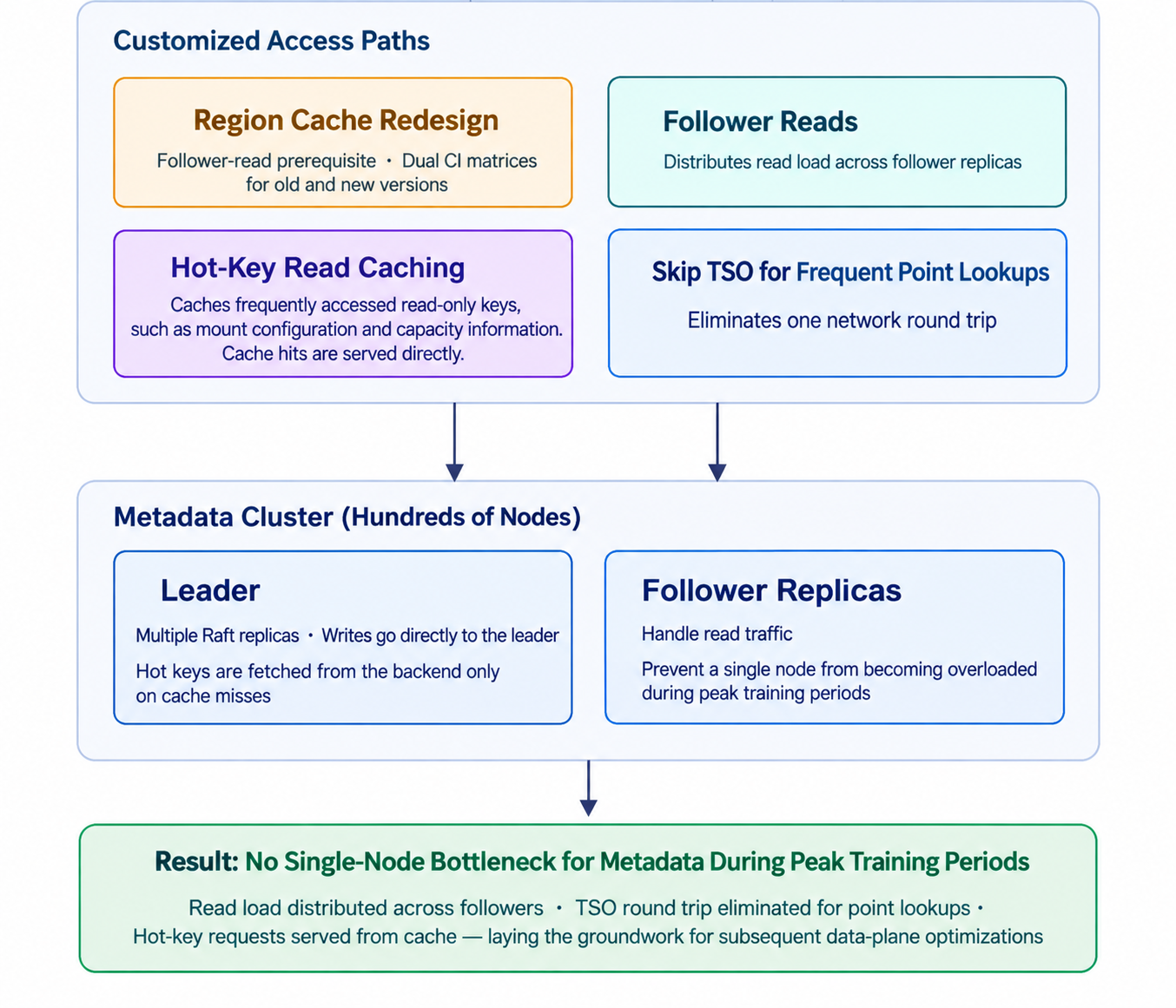
- During peak training periods, the CPU on nodes hosting the leader replica was saturated, while follower replicas still had spare capacity.
- Transactions requested global timestamps from the Timestamp Oracle (TSO) service in Placement Driver (PD), adding a network round trip.
- Hot metadata, including mount configuration and capacity information, was queried repeatedly.
Further parameter tuning alone could no longer relieve these bottlenecks. We needed to change the access paths.
To address them, we modified the Region routing cache in the TiKV Go client so follower replicas could handle read requests. We also eliminated one TSO round trip from frequent point lookups and introduced a read cache for hot metadata.
We validated the changes against both old and new versions through continuous integration tests. Then, we delivered them as build-time patches, avoiding the need to maintain a long-lived fork of the upstream dependency. When scaling the cache cluster in or out, we also minimize large-scale cache-key remapping to reduce the risk of cache stampedes.
Large directories containing billions of entries also put pressure on client memory. We adopted streaming, batched directory scans to avoid building the entire result set in memory during a single readdir call. This prevents out-of-memory failures and supports kernel-level readdir caching.
Rate limiting to keep the cluster stable
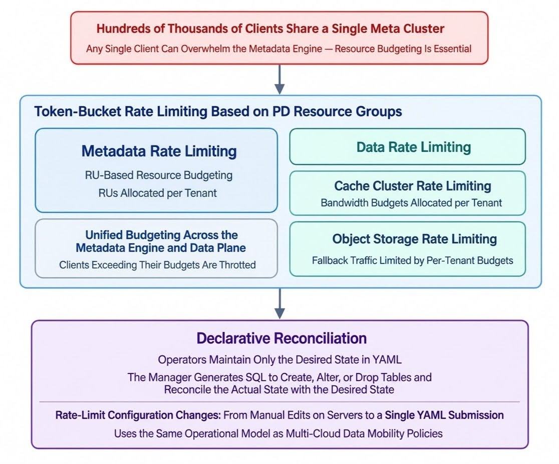
Hundreds of thousands of clients share one Meta cluster, and a single client can overwhelm it. To prevent one tenant's traffic from affecting the entire cluster, we independently limit resource consumption in the metadata and data planes.
On the metadata side, we use token buckets based on PD Resource Groups. Request Units (RUs) measure and limit each tenant's resource consumption. In the data plane, we separately limit traffic to the cache cluster and traffic that falls back to object storage.
Clients that exceed their budgets are throttled before their load can overwhelm shared resources. We manage rate-limit budgets declaratively: operators maintain the desired state in YAML files, and the manager compares that state with the current configuration and automatically generates SQL statements to create, alter, or delete database tables as needed.
Metadata disaster recovery: cold backups as a last line of defense
Metadata is critical to the entire system. TiKV stores the relationships between hundreds of billions of files and their metadata. If that metadata cannot be recovered, the file contents may still exist in object storage, but the system may no longer know which files they belong to.
We use three layers of protection against different failure scenarios:
- TiKV Raft replication protects against hardware failures.
- Periodic full snapshots of TiKV are backed up to object storage in a separate region. These backups provide a recovery path for accidentally deleted metadata in a keyspace, logical metadata corruption, and region-wide failures.
- Object storage retains the file contents, allowing datasets to be used again after metadata recovery. When recovery is needed, we rebuild the TiKV cluster and restore the latest snapshot.
Cold backups come with a trade-off: metadata can only be restored to the most recent backup. Changes made afterward may be lost, and the potential recovery point depends on the backup interval. For our current training workloads, this is an acceptable trade-off.
Challenge 2: Data visibility and governance, reducing costs by deleting 200 PB every week
When approximately 200 PB of data is deleted each week, logical deletion is only the beginning. Object storage continues to accumulate billions of objects awaiting reclamation, and a single-node scan cannot keep up. Failed asynchronous deletions can also leave orphaned objects whose keys no longer reveal which files they belonged to.
We built a governance workflow that connects deletion decisions, recovery from accidental deletion, space reclamation, and leak auditing.
Deletion decisions: dashboards and application-owner review
Application owners must decide what to delete and when. A trash cannot replace that decision-making process.
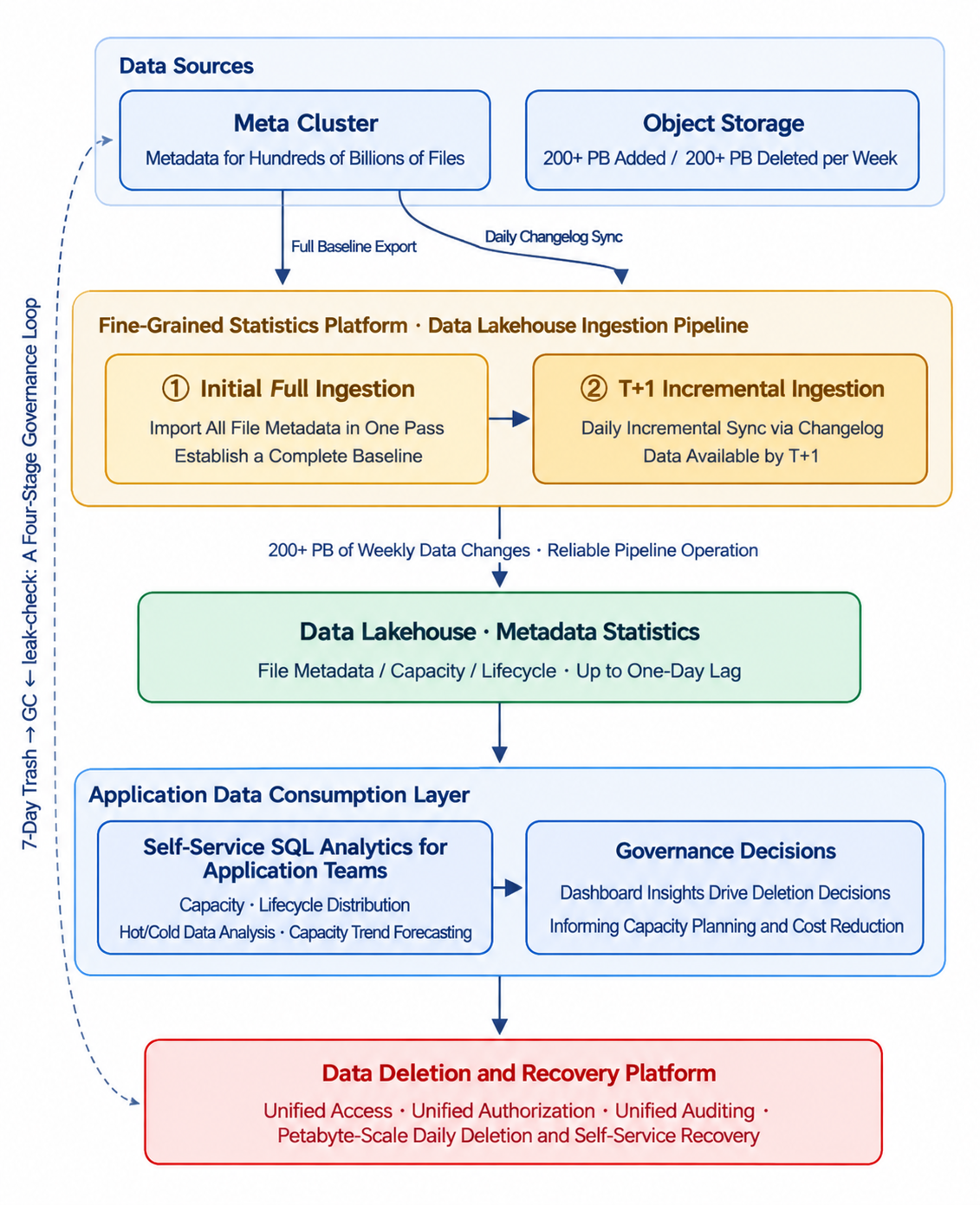
We provide dashboards showing dataset access patterns, changes in access frequency, and capacity growth trends. Application owners use this information to plan deletions and capacity expansion. Once they confirm a decision, they can initiate deletion or recovery themselves. Deleted data first enters the trash.
The dashboards rely on a metadata statistics pipeline that makes data queryable the next day (T+1). We first export the full set of file metadata from the Meta cluster to the data lakehouse to establish a baseline. After that, we synchronize incremental changes daily through the changelog.
Application owners can query capacity, access patterns, and lifecycle data directly without asking the storage team to run queries for them. With approximately 200 PB of data added and deleted every week, any interruption or data drift in this pipeline can undermine capacity planning and reclamation decisions. Keeping the pipeline reliable is therefore essential.
Recovering deleted data: a seven-day trash
Data deleted through the platform remains in the trash for seven days. This window provides time to recover accidentally deleted data and absorbs the daily deletion volume, which can reach petabytes. It also prevents reclamation workloads from placing immediate pressure on the metadata engine.
The trash uses different mechanisms for different paths:
| Mechanism | Design | Purpose |
|---|---|---|
| Paths that bypass the trash (mount options) | Skip the trash for paths explicitly designated as non-recoverable, such as temporary training directories. | Prevent large volumes of data from overwhelming the trash. |
| Scheduled batch cleanup | Delete data older than seven days in batches organized by time bucket. The process is observable and supports recovery. | Manage trash capacity while preserving recovery capabilities. |
| Streaming deletion lookup | Scan deleted files as a stream to locate the requested data. | Enable recovery within seconds and support deletion audits. |
During the retention period, application owners can restore data themselves through the recovery platform or command-line tools, without filing an operations ticket. Recovery rolls back metadata and rebuilds object references without copying the underlying data. The platform supports petabyte-scale daily recovery, and a single PB-scale recovery can finish within hours. Both deletion and recovery enforce permissions through access control lists (ACLs) and record audit logs.
Reclaiming space: distributed garbage collection
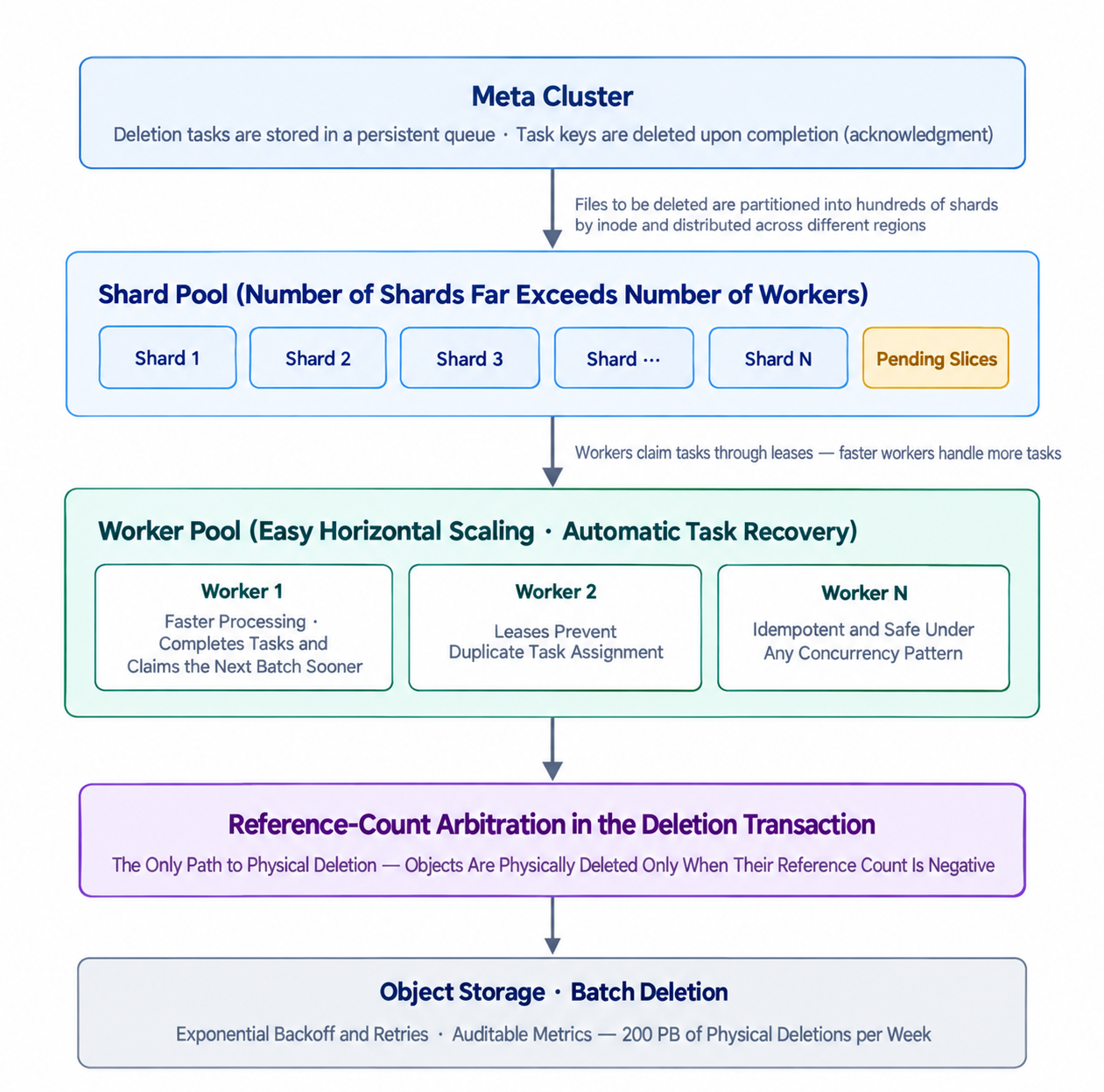
The standard Community Edition garbage collection (GC) relies on single-node scans. This cannot keep pace with approximately 200 PB of weekly deletions. We modified the process to record files and data slices awaiting deletion in TiKV, and then divide reclamation work into multiple shards for parallel processing by multiple workers.
Workers acquire tasks through leases. After completing a task, a worker deletes its task record and claims the next batch. Tasks remain in TiKV until completion. If a worker fails, another worker can take over unfinished work. This approach distributes reclamation load without requiring a separate message queue.
Leases determine which worker handles a task. Reference counts in the deletion transaction determine whether an object can actually be deleted. Physical deletion proceeds only when the reference count meets the deletion condition—in the current implementation, a negative value. This prevents concurrent processing or retries from causing duplicate deletions.
On the object storage side, reclamation uses batch deletion, exponential backoff and retries, and audit records.
We apply the same distributed processing model to large-file compaction. Files that grow through repeated appends can accumulate many slices, increasing read overhead. A separate gc_cluster distributes compaction tasks from a manager to multiple workers.
These workers periodically merge slices online to control read amplification.
Auditing orphaned objects with leak-check
In addition to reclaiming objects based on metadata records, we use leak-check to identify objects that were missed by the deletion process.
The standard [fsck](https://juicefs.com/docs/cloud/reference/command_reference/#fsck) check in JuiceFS looks for cases where metadata references an object that is missing. leak-check performs the reverse check: it finds objects that still exist in storage but are no longer referenced by metadata.
On the object storage side, we list objects concurrently across 32 subprefixes under chunks/, reducing the bottleneck caused by scanning through a single connection. We independently obtain the object inventory and the metadata reference inventory. We then use two external-sort (extsort) operations and merge the sorted results as streams to generate a candidate list. This avoids building a full in-memory map containing hundreds of billions of entries.
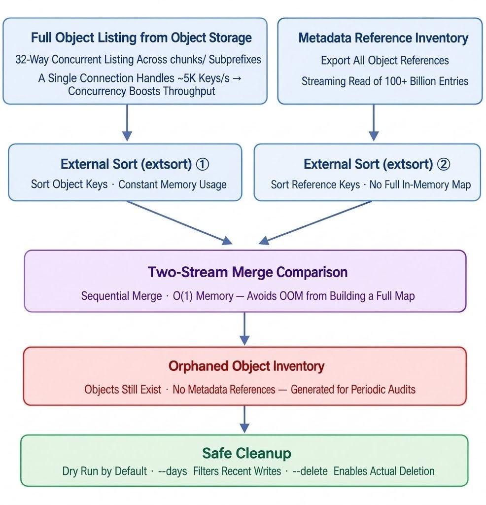
The comparison results are only candidates for cleanup; they cannot be deleted immediately. Objects being written may temporarily lack metadata references. By default, the audit generates a list without deleting anything and filters out recently created objects. Deletion happens only after the candidates are reviewed and confirmed. This process helps find orphaned objects while reducing the risk of deleting writes that are still in progress.
Challenge 3: Balancing training performance and EB-scale storage costs
Training requires throughput on the order of hundreds of GB/s. It also combines large sequential I/O for datasets with small random I/O for checkpoints. At EB scale, we cannot keep all data in the hot tier. When compute runs across multiple clouds, data must also be accessible from locations close to the workloads.
Three-tier caching: from clients to a centralized cluster
Our three-tier cache expands the sharing scope at each level:
- L1 cache: Reuses data blocks within the current client.
- L2 cache: Shares data blocks between clients through peer-to-peer (P2P) transfers.
- L3 cache: A centralized cluster that serves hot training data for both reads and writes.
Reads check L1, L2, and L3 in sequence. Only when all three tiers miss does the client access object storage.
When multiple training jobs read the same dataset, L1 caching alone cannot share data across clients, so clients may fetch the same data from object storage repeatedly. L2 allows clients to act as cache peers. A block already cached by one client can be reused by another through the range-read (getrange) interface. When dozens of jobs read the same data concurrently, the total amount fetched from object storage can approach the size of a single copy. This saves bandwidth by making better use of existing local disks and memory.
Requests that miss both L1 and L2 proceed to the centralized L3 cache cluster, which handles PB-scale data. L3 serves hot working sets shared across clients and absorbs most of the read throughput. The same cluster provides both read caching and write aggregation: read caching serves large sequential dataset I/O, while write aggregation handles small random checkpoint I/O. The cluster can scale horizontally to increase hot-data capacity.
A cache failure could force hundreds of thousands of clients to fetch data directly from object storage at once, increasing the load on the storage backend. We use health checks to remove unhealthy nodes and reintroduce them after recovery. If the read cache becomes entirely unavailable, clients fall back to direct reads from object storage, trading higher latency for continued access.
We also record cache hit counts, bytes served, latency, and slow requests at each tier. These metrics help us detect cache degradation and changes in fallback traffic.
Metadata caching: avoiding repeated lookups
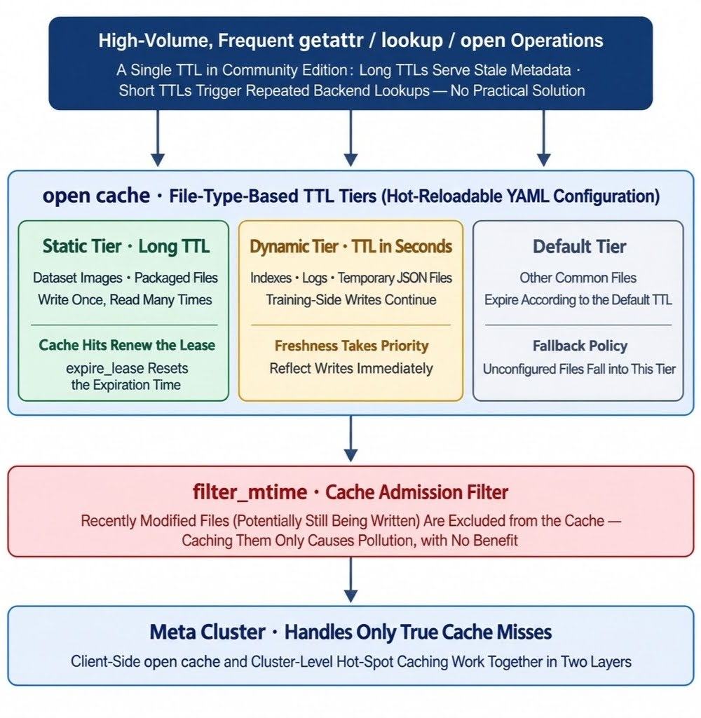
When a training job reads a file, it must do more than retrieve data blocks. It also repeatedly looks up files, retrieves file attributes, and opens files through operations such as lookup, getattr, and open. Each operation requires a metadata query.
To reduce repeated requests to TiKV, the client uses an [open cache](https://juicefs.com/docs/community/command_reference#mount-metadata-cache-options) to retain query results.
The challenge is that different file types change at different rates. Dataset images and packaged files usually remain unchanged for long periods and can be cached longer. Indexes and logs, by contrast, may change continuously and need to reflect updates quickly.
Using the same time-to-live (TTL) for every file creates a trade-off: a long TTL risks serving stale metadata, while a short TTL forces frequently accessed but unchanged files to query the backend repeatedly.
Therefore, we define three TTL tiers by file type. Static files use longer TTLs, dynamic files use TTLs measured in seconds, and other files use the default TTL. The configuration supports hot reloading through YAML.
For static files, a cache hit renews the lease (expire_lease), resetting the expiration time. Frequently used files can therefore remain cached, while cold files expire naturally. The modification-time filter (filter_mtime) prevents recently modified files—which may still be receiving writes—from entering the cache. This avoids caching metadata before it has stabilized.
Controlling read amplification: coordinating prefetching and caching
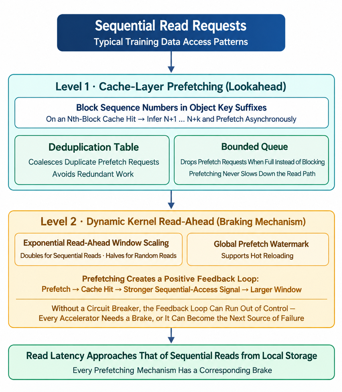
Prefetching can accelerate sequential reads, but excessive prefetching can also increase load on the storage backend. We control prefetching independently at the cache layer and the kernel layer.
At the cache layer, the client uses block sequence numbers in object keys to fetch subsequent blocks in advance. A deduplication table and bounded queue limit concurrency. When the queue is full, the client drops prefetch requests rather than blocking normal reads.
At the kernel layer, dynamic read-ahead adjusts the window based on whether access is sequential or random. A global watermark limits the overall load, and the configuration supports hot reloading.
Keeping data close to compute and tiering by access frequency
The changes described above improve access to hot data. Controlling storage costs at EB scale also requires deciding where data should reside.
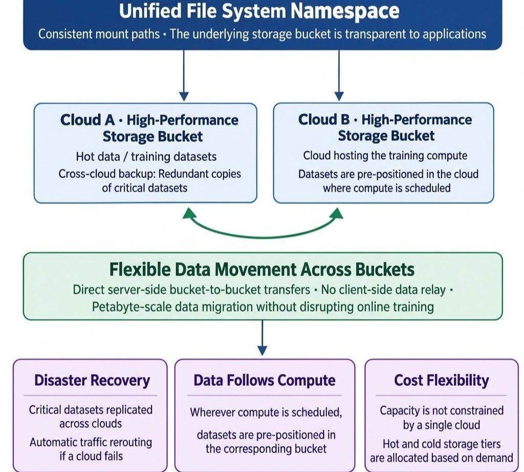
When training workloads run across multiple clouds, we allow buckets in different regions to share a single file-system namespace. Metadata records each object's owning bucket and storage tier. Read requests use this information to route to the appropriate bucket, so migrating data does not require application access paths to change.
Data moves directly between buckets on the server side, without consuming client bandwidth. During migration, the read path falls back across the hot tier, cold tier, and full pool as needed. Declarative configuration controls the owning bucket and migration policy for datasets or directories.
When training compute moves to another cloud, we can migrate data to the corresponding region in advance, reducing dependence on cross-cloud dedicated bandwidth. Infrequently accessed data can be moved to lower-cost buckets or cold-storage pools such as tape libraries and retrieved when needed.
This approach keeps hot data close to compute while controlling storage costs at EB scale. Capacity scaling no longer depends on a single cloud provider. Critical datasets can also retain backup buckets in other clouds, providing an alternative read path during cloud outages.
Challenge 4: Connecting and managing hundreds of thousands of clients
When hundreds of thousands of clients connect simultaneously, multi-tenant access control, connection methods, and client observability all need to be designed for scale. We address these concerns through access control, training-job integration, and client monitoring.
Multi-tenancy: access control
Our production kernel versions do not support enabling POSIX-compliant ACLs on the Filesystem in Userspace (FUSE) mount path. Therefore, we moved tenant authorization into a user-space ACL Manager.
The ACL Manager uses buckets as the unit of authorization and manages permissions through the READER and MAINTAINER role groups. It supplements lightweight directory access protocol (LDAP) group information using globally unique identifier (GUID) files and records audit logs.
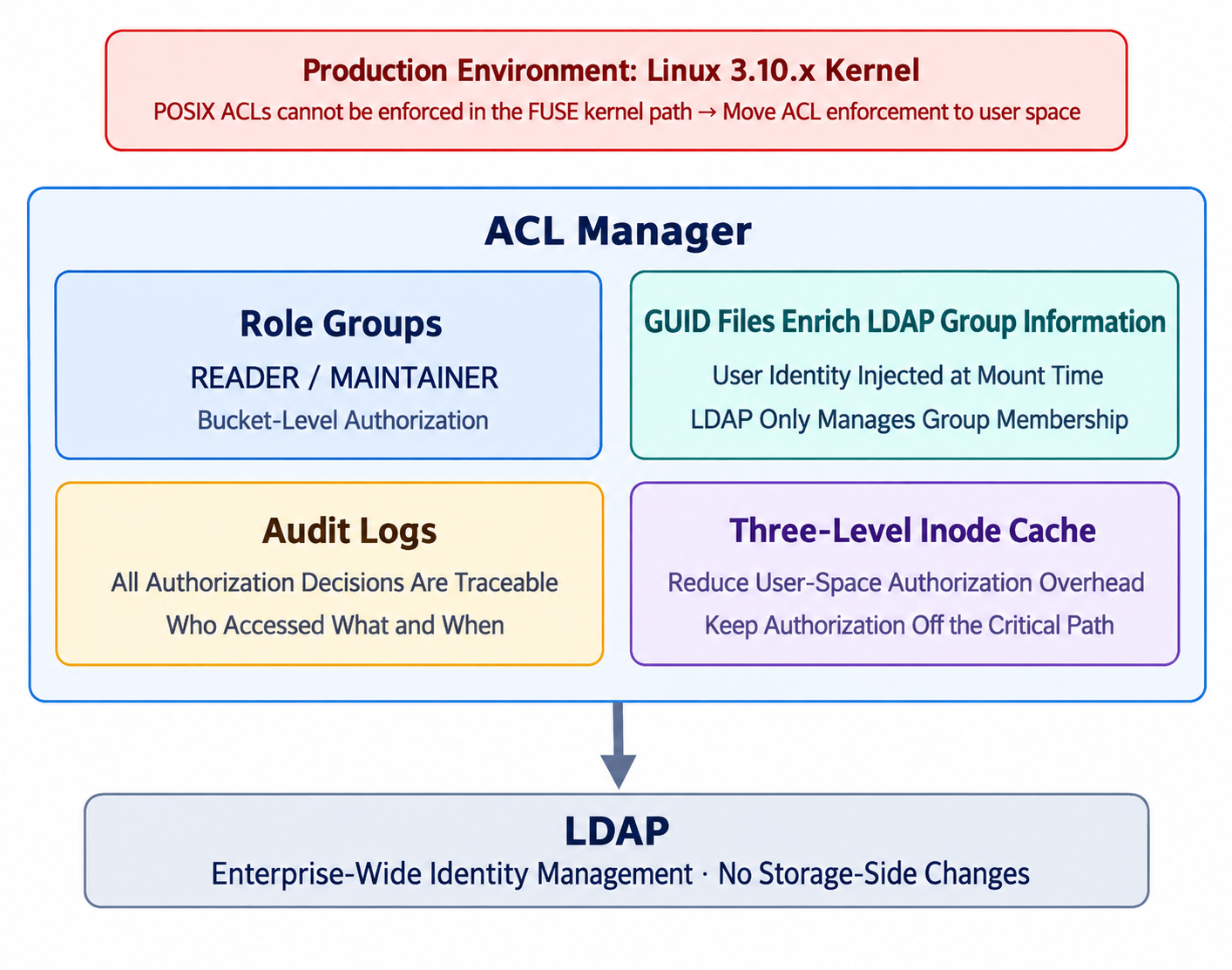
With this design, LDAP only needs to maintain group membership. The ACL Manager implements ACL semantics in user space, bypassing kernel-version limitations and rejecting unauthorized access to shared file systems during authorization.
The trade-off is additional user-space authorization overhead, which we mitigate with a three-level inode cache.
Access methods: S3 Gateway and a mountless SDK
In addition to POSIX mounts, we provide two access paths: an S3 Gateway built on the MinIO plugin layer and an in-process SDK for direct data access.
Some applications already use the S3 protocol and need to keep their existing interfaces while accessing the same data. The S3 Gateway translates object-protocol requests into file-system operations. It shares the same file-system namespace with POSIX mounts and the SDK, reusing the same permissions, caches, and underlying data.
The plugin layer implements directory-level tenant isolation and user-token validation, and fixes slow paginated queries in ListObjectsV2. We also removed support for non-S3 backends to create a lightweight image. For cross-cloud dedicated-network scenarios, we provide a lightweight SDK for read-side access via the S3 protocol.
The other access path targets highly concurrent training workloads. As the number of jobs and dataloader processes grows, the number of simultaneously active client data connections can reach the millions. FUSE access requires requests to pass through the kernel, while short-lived jobs repeatedly mount and unmount the file system. The resulting connection and mount overhead accumulates.
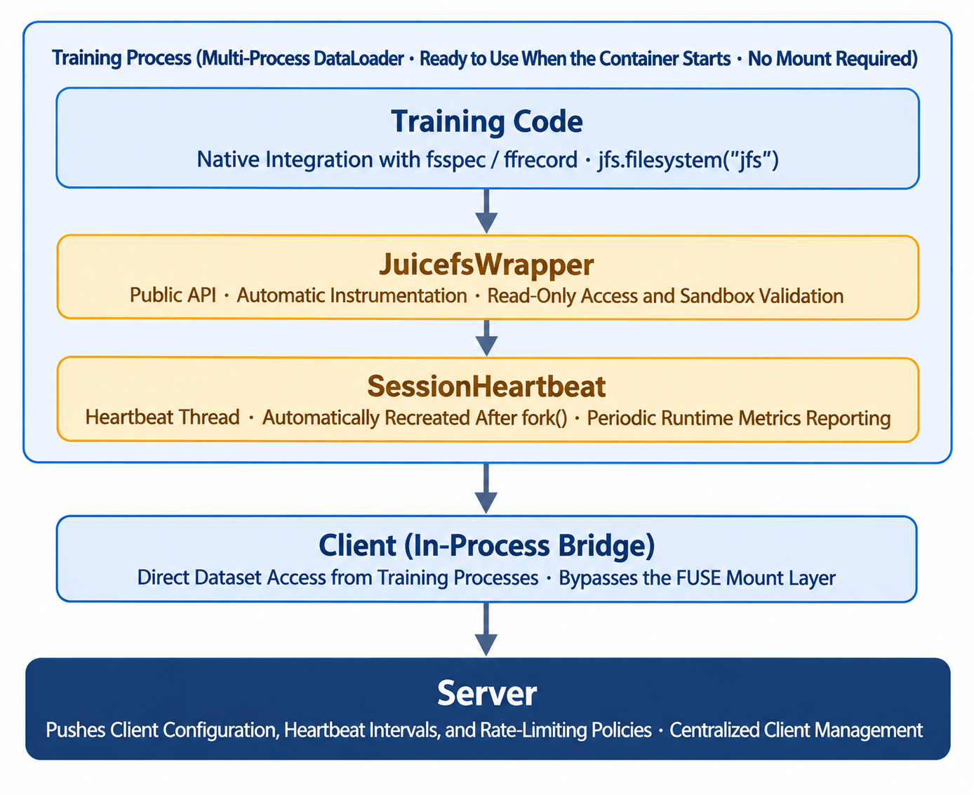
To address this, we developed an in-process Python SDK that reads data directly without requiring a mount. Connections are created and exit with the process. The trade-off is that the SDK must manage process connections, sessions after fork, and heartbeats itself.
The SDK starts with the container and integrates with existing data-loading pipelines through fsspec and ffrecord. When dataloader processes are forked, each child process recreates its session and heartbeat thread and reports metrics independently. During operation, the SDK periodically reports metrics and receives heartbeat intervals and rate-limit policies from the server.
Training workloads use read-only access, and write operations are blocked at multiple layers. Path validation and cross-bucket isolation further prevent unauthorized access.
Metric observability and client upgrades
Each of hundreds of thousands of clients can generate hundreds of metrics. If Prometheus scraped every client individually, the number of time series would grow rapidly.
Instead, clients report metrics to MetricManager in shards, and Prometheus scrapes the aggregated results. MetricManager controls time-series cardinality by merging or dropping some fine-grained labels. The trade-off is that some observability dimensions are no longer available.
The aggregation service must also support hot configuration updates, recovery from failures, dropping data under overload, and expiration-based cleanup. Otherwise, the service itself could become a bottleneck.
Rolling out upgrades across hundreds of thousands of clients must also minimize disruption to training workloads. The Gateway and file-system client (FS) images are produced through the same build pipeline. Combined with stateless clients and rolling restarts in K8s, this supports staged upgrades.
Upgrades to the direct-read SDK and S3 Gateway are transparent to training jobs. For POSIX mounts, the disruption window can be kept under control.
We are evaluating several general-purpose improvements for potential upstream contributions, including batched cache APIs, streaming scans through ReaddirFrom, and dynamic read-ahead. Features more tightly coupled to our application requirements, such as ACLs and the end-to-end data governance workflow, will continue to evolve internally.
Conclusion
Our experience managing EB-scale capacity, hundreds of billions of files, and hundreds of thousands of clients comes down to four principles.
- Distribute the workload to eliminate centralized bottlenecks. We distribute metadata reads across follower replicas, eliminate the extra TSO round trip for frequent point lookups, and optimize hot keys to prevent individual nodes from becoming overloaded. We also customize the metadata access path to improve overall performance. When designing the architecture, we must account for the impact of failures in components that carry global workloads.
- Govern the data lifecycle with an end-to-end workflow. Dashboards support deletion decisions by application owners; a seven-day trash and PB-scale recovery protect against accidental deletion; GC reclaims space; and
leak-checkaudits orphaned objects. Recovery throughput must keep pace with deletion volume so that reclamation anomalies remain within an acceptable space-reclamation delay, reducing both accidental data loss and the risk of permanent storage leaks. - Protect training performance through tiered caching and bounded prefetching. L1 client caching, L2 P2P caching between clients, and the centralized L3 cluster absorb load at progressively broader sharing scopes. Prefetching is constrained by global limits and queue watermarks. When queues fill, requests are dropped rather than allowed to slow normal reads through additional read amplification. Data locality and hot/cold tiering further reduce cross-cloud access costs and EB-scale storage expenses.
- Limit the impact of individual tenants through access control and resource budgets. ACLs define the scope of access, while token buckets constrain each tenant's resource consumption in both the metadata and data planes. Declarative RU-based resource budgets make these limits manageable and help prevent a single client from destabilizing the shared cluster.
As data volumes, compute capacity, and application complexity continue to grow, we’ll keep improving the metadata engine, data plane, performance engineering, governance mechanisms, and observability. Our goal is to prepare the architecture for the next order-of-magnitude increase before it arrives. Identifying potential bottlenecks early and addressing them proactively will remain a central focus of our work.
If you have any feedback on this article or ideas to share, we invite you to participate in the discussions on GitHub and join our community on Discord.
