Optimizing JuiceFS on the Arm Architecture: MLPerf-Based Performance Tuning

Recently, building high-performance storage infrastructure on Arm platforms has become a technical focal point. Linaro is an international technology organization focused on the Arm ecosystem and open-source software. We collaborate with upstream and downstream industry players to address common issues and assist enterprise customers in productizing their solutions on an open-source foundation. Our team conducted systematic stress testing on JuiceFS Community Edition (using Redis for metadata storage) during MLPerf Storage benchmarks, covering a variety of typical machine learning training workloads.

Our test results show that system performance is largely influenced by memory bandwidth and metadata access efficiency. JuiceFS’ throughput directly determines GPU utilization and training efficiency. Through testing workloads such as 3D U-Net, ResNet-50, and CosmoFlow, the analysis revealed: in single-node scenarios, GPU utilization is primarily limited by memory copy latency; in two-node or multi-node scenarios, metadata access and inter-node synchronization become the main bottlenecks. In the article, we also provide tuning strategies and practical results to address these bottlenecks.

In summary, large-scale AI training performance tuning is a systematic engineering effort that requires coordinated optimization across storage systems, memory bandwidth, CPU scheduling, caching strategies, and more to achieve efficient deep learning data supply on Arm platforms.

Arm64 vs. x86_64 architecture differences and concurrency characteristics

Compared to x86, Arm’s application scope continues to expand, extending from mobile devices to IoT, wearables, PCs, automotive, and servers. Its high performance per watt is a key reason for its widespread adoption.
From an architectural design perspective, Arm is a reduced instruction set computer (RISC), while x86 is a complex instruction set computer (CISC). This design difference also affects how processors execute instructions. Arm64 instructions have a fixed length of 4 bytes, whereas x86 instructions have variable lengths ranging from 1 to 15 bytes. Consequently, x86 often requires more complex decoders. In contrast, Arm’s instructions are simpler and rely more heavily on effective instruction organization during compilation and code generation, thus requiring longer compilation times.

From an engineer’s perspective, there are other architectural differences that directly impact program behavior. Code that seems intuitive on x86 may not behave the same way on Arm. Several of the common pitfalls discussed later are fundamentally related to these underlying differences.

One typical issue is the alignment requirement for atomic operations. Whether using Load-Link/Store-Conditional (LL/SC) or Large System Extensions (LSE), read-modify-write operations like atomic increments typically require aligned memory addresses. Newer LSE2 relaxes this restriction, supporting unaligned accesses within a 16-byte window. Data alignment is not mandatory for x86, but maintaining good alignment helps improve performance. See Arm Architecture Reference Manual for A-profile architecture.

Another key feature to note is that Arm employs a weakly ordered / relaxed memory model. The difference lies in the strength of constraints on memory access ordering. In multi-threaded scenarios, the same read/write operations are more likely to appear in program order on x86, whereas Arm permits more reordering. Thus, the order observed by other threads may differ from the source code order. When debugging issues on Arm, memory ordering effects must be carefully considered. For more details, see the Arm white paper: Synchronization Overview and Case Study on Arm Architecture.

Overview of JuiceFS and MLPerf

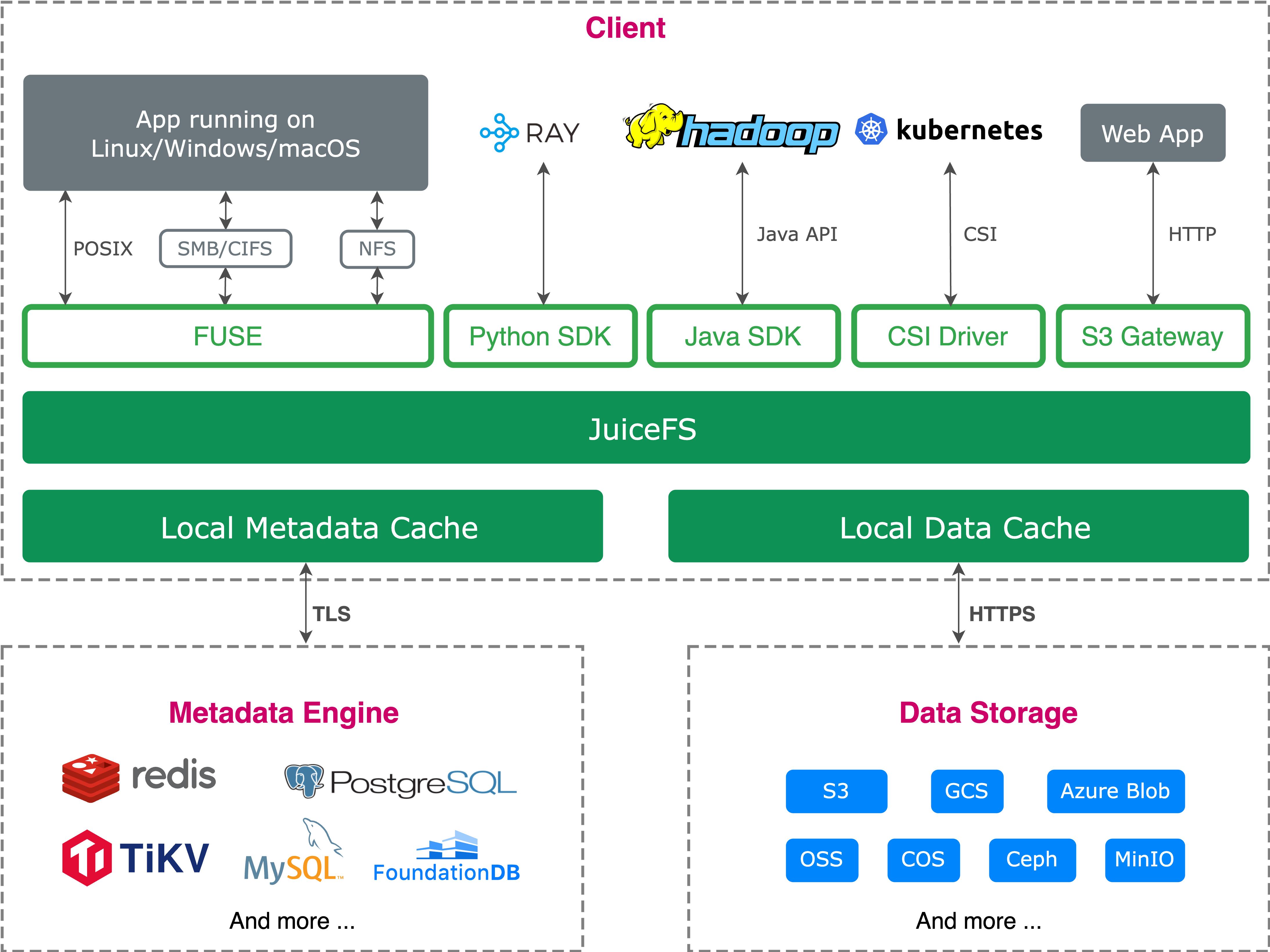
JuiceFS is an open-source, high-performance distributed file system built on object storage. It leverages the cost advantages of object storage while delivering a user experience close to traditional file systems. It supports POSIX, HDFS SDK, Python SDK, and S3-compatible interfaces, adapting to various applications and data processing frameworks. It also supports cloud-native extensions, data security, and compression, making it widely applicable to AI training, inference, big data processing, and more.

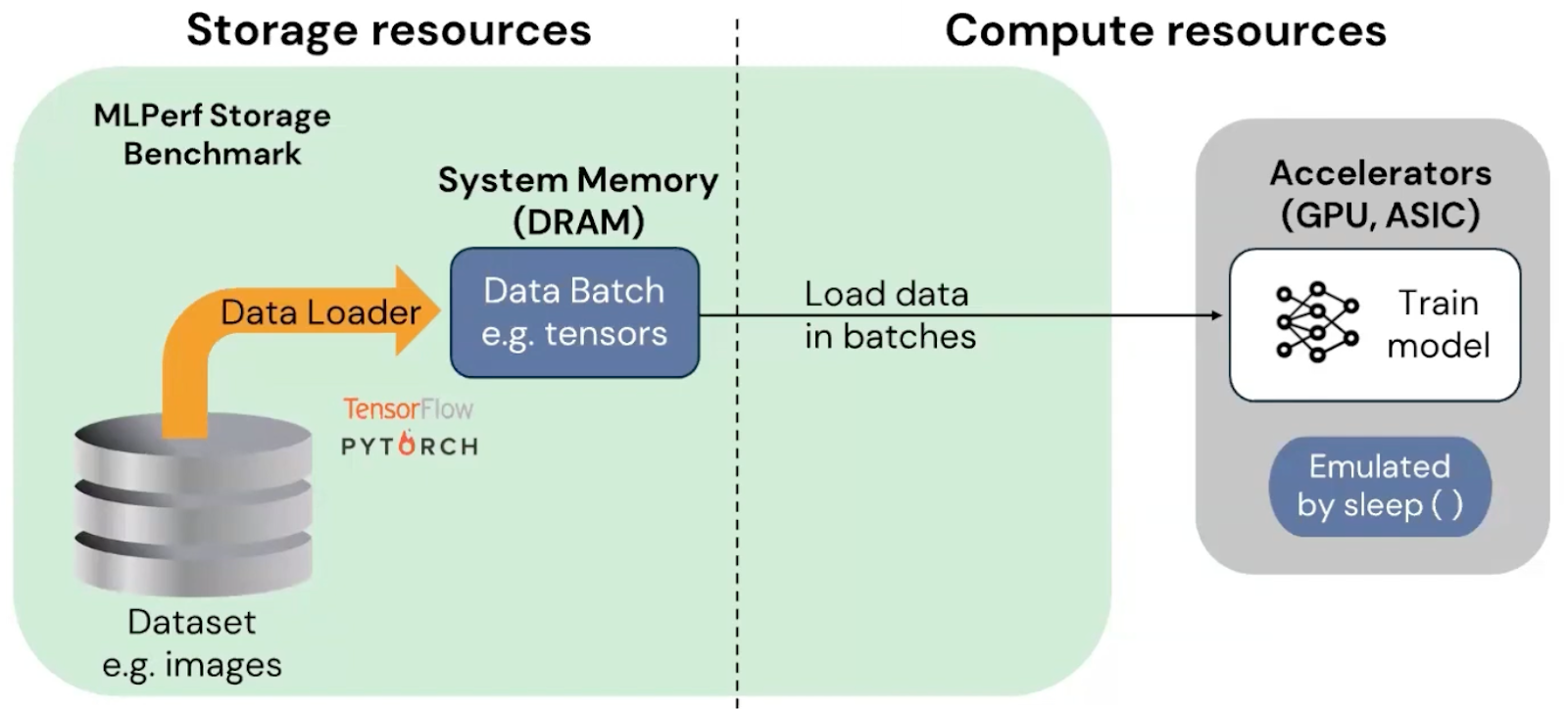
To evaluate JuiceFS’ data supply capability under high-load scenarios like AI training, we can use the MLPerf Storage benchmark. Developed by MLCommons, this benchmark focuses on measuring a storage system’s ability to consistently and efficiently supply data to compute nodes.

Version 2.0 divides tests into training workloads and checkpoint workloads. The training workloads include 3D U-Net, ResNet-50, and CosmoFlow. They differ significantly in sample size and access patterns. Minimum GPU utilization requirements are set: 90% for 3D U-Net and ResNet-50, and 70% for CosmoFlow.

The table below shows MLPerf Storage 2.0 training workloads:

Task	Reference network	Data loader	Sample size	Batch size	Accelerator utilization	Time per batch run (s)	Evaluate storage capability
Image segmentation (medical)	3D U-Net	PyTorch	146 MiB	7 x 146 = 1,022 MiB	90%	0.323 / 0.9 = 0.359 Data load time: 0.359-0.323 = 0.036	Bandwidth, concurrent large block sequential reads
Image classification	ResNet50	Tensorflow	150 KiB	400 x 150 = 58.5 MiB	90%	0.224 / 0.9 = 0.249 Data load time: 0.249 - 0.224 = 0.025	Bandwidth, IOPS, high concurrency medium block sequential reads
Scientific (cosmology)	Parameter prediction	Tensorflow	2.7 MiB	1 x 2.7 = 2.7 MiB	70%	0.0035 / 0.7 = 0.005 Data load time: 0.005 - 0.0035 = 0.0015	Bandwidth, IOPS, metadata latency, high concurrency sequential reads of many small files
LLM checkpointing (new)	Llama3	PyTorch	105GiB to 18TiB	—	—	—	Bandwidth, concurrent sequential writes of extremely large files

In the test flow, data is first read from the storage system into host memory before entering the compute phase. Training time is simulated to replicate the data flow of real training scenarios, eliminating the need for actual GPU deployment, lowering experimental barriers, and improving operational convenience.

MLPerf Storage v2.0 test principles and tuning

Before detailing specific model test results, it’s essential to understand the data access principles of distributed training. This helps readers grasp the causes of GPU utilization, storage throughput, and performance bottlenecks, enabling better comprehension of subsequent test results and tuning strategies.

Distributed machine learning typically uses data parallelism, where multiple parallel processes share the same dataset, and each process handles reading and processing its corresponding training batches.

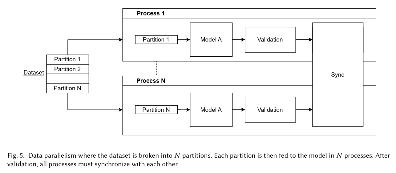
MLPerf Storage training tests follow this approach: each training process reads data from the storage system in batches and simulates computation to evaluate the storage system’s ability to sustain data supply.

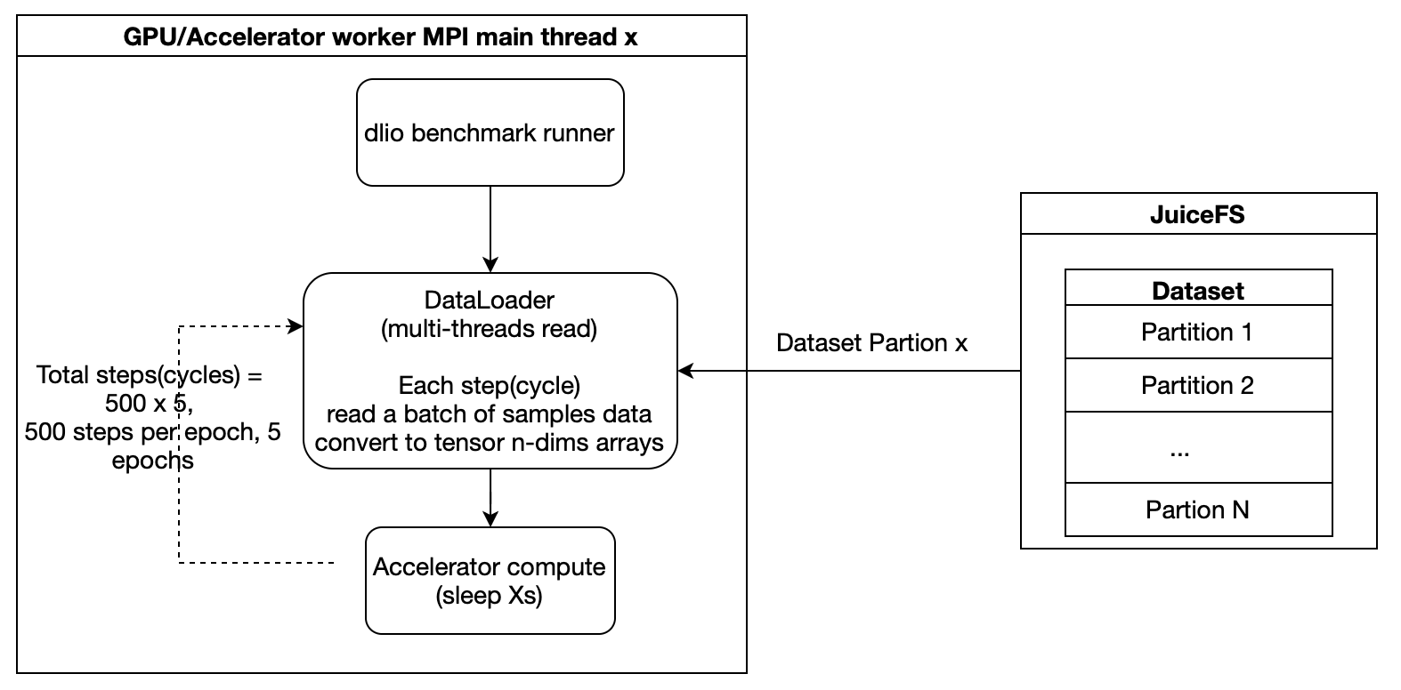
To understand the source of performance during testing, it’s also necessary to understand the data processing path within the JuiceFS client.

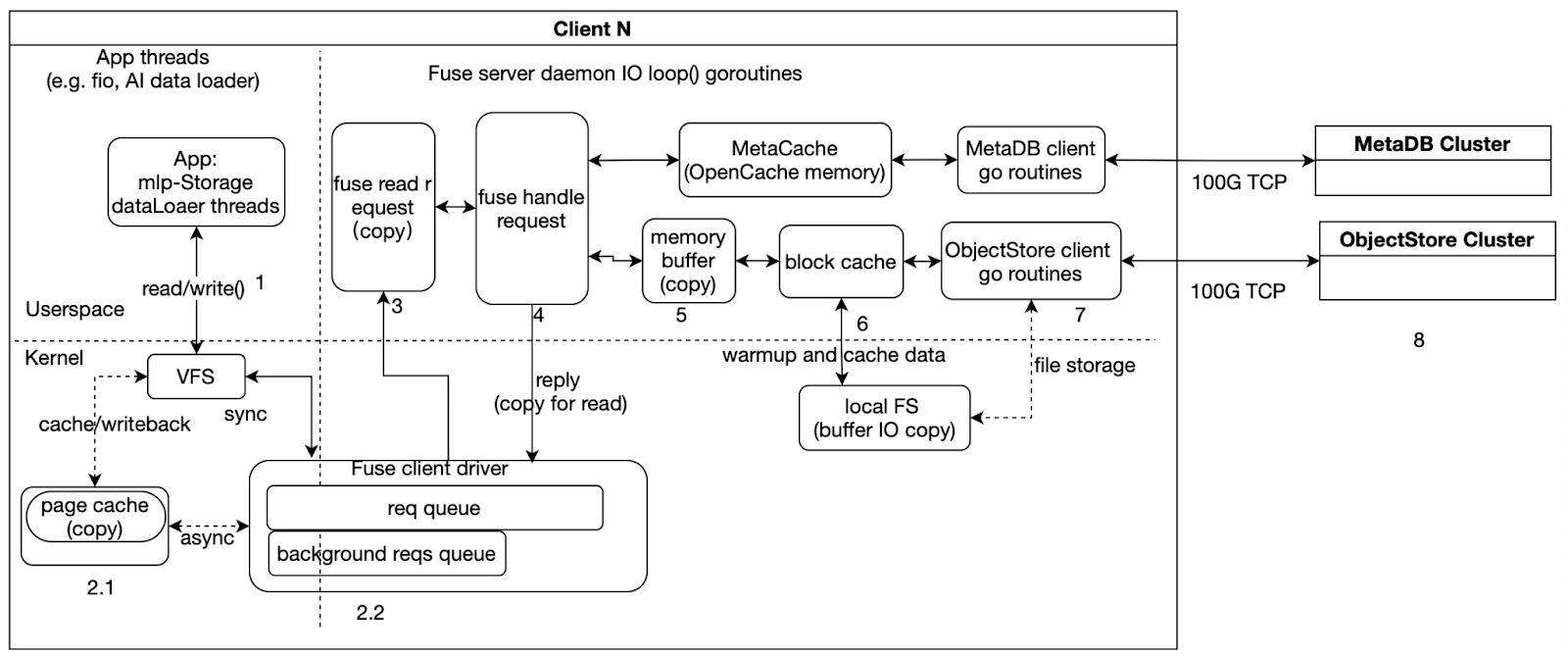
As illustrated, when testing with JuiceFS, the execution flow can be roughly divided into three parts:

• Left side: Application-side I/O threads, such as fio or MLPerf Storage’s DataLoader threads, which initiate read/write requests and wait for completion.
• Middle: The main goroutine in the FUSE daemon, which handles FUSE requests from kernel space, places file data into memory buffers and caches, and triggers backend metadata and object storage access.
• Right side: Asynchronous goroutines for the Meta client and ObjectStore client, which interact with the backend MetaDB and ObjectStore clusters for data and metadata operations.

From a performance analysis perspective, we need to note two types of issues:

• Data copying, corresponding to steps like 2.1, 3, 4, 5, and 6 in the diagram. These steps introduce additional memory copy overhead and are often key areas for analyzing latency and CPU usage.
• Synchronization and asynchronous boundaries. As shown, steps 1, 2, 3, 4, 5, and 6 are part of the synchronous path, where the request must wait for the current stage to complete before proceeding. Step 7 is part of the asynchronous path, handled by background goroutines interacting with backend storage.

Test 1: 3D U-Net

In this test, the sample size was 146 MiB per image file, and we focused on large-block read performance. The test results showed:

• In a single-node environment, the system could stably run up to 5 GPUs, with GPU utilization at about 50%.
• In a two-node scenario, it could support 10 GPUs, also with GPU utilization around 50%.

To improve data read efficiency, we optimized the training parameters: we increased the number of reader threads from 4 to 16 to accelerate data generation, and switched to direct I/O to reduce buffer and memory copy overhead.
Operational metrics showed that when mounting 6 GPUs on a single node, GPU utilization dropped to 83%, corresponding to a bandwidth of about 15.1 GB/s. This fell short of the expected high utilization target. Further testing with fio on the storage side revealed similar bandwidth of about 15.1 GB/s. This indicated that the bottleneck had shifted to the JuiceFS client bandwidth rather than the GPU compute side.

Optimization analysis 1: CPU pinning

To further investigate the cause of the client bandwidth limitation, we pinned the process to a specific CPU (running on NUMA nodes 2 and 3). Monitoring showed that all 48 CPU cores were nearly fully utilized. Further analysis of top-down, memory, and miss metrics revealed a clear memory-bound condition, with most time spent on memory copying. This indicated that in the CPU-pinned scenario, the performance bottleneck of JuiceFS primarily came from CPU processing capacity and the additional latency caused by cross-NUMA node memory copying.

Optimization analysis 2: no CPU pinning

To understand the bandwidth limitations under more general conditions, we observed the scenario without CPU pinning. The results showed that while the CPU was not fully saturated, the devkit tuner numafast metric indicated that remote memory access accounted for about 80% of total memory accesses. This meant a large number of memory accesses were crossing local NUMA nodes, potentially even across CPU sockets, introducing significant bandwidth loss and access latency.

From the perspective of hardware bandwidth, cross-socket memory access has inherent limitations. For example, on the Arm platform, the theoretical physical bandwidth across sockets was about 60 GB/s. Further measurements showed cross-socket copy bandwidth on Arm1 to be around 48 GB/s, while on two x86 platforms it was about 37 GB/s and 28 GB/s, respectively.

This suggested that in the scenario without CPU pinning, even though the compute cores were not fully exhausted, extensive cross-node, cross-socket remote memory access had become a major source of overhead. Therefore, we inferred that the inability to further increase JuiceFS bandwidth was likely not solely due to CPU compute power, but rather constrained by the bandwidth and latency of cross-socket memory access. In other words, the system bottleneck had shifted from “local CPU being too busy” to “remote memory access being too costly.”

In summary, the reasons for the JuiceFS bandwidth limitation differed between the two scenarios:

• With CPU pinning, the bottleneck was primarily CPU resource consumption and the overhead of extensive memory copying.
• Without CPU pinning, the bottleneck was largely due to a high proportion of non-local memory accesses, especially the bandwidth and latency penalties from cross-socket accesses.

Test 2: ResNet-50

ResNet-50 uses small samples (about 150 KiB each), with each batch containing 400 samples totaling about 58.5 MiB. This I/O test focused on data loading efficiency and training throughput under high GPU concurrency. The system maintained high utilization at large GPU scales:

• Single node: 50 GPUs, 95% GPU utilization, about 9.2 GB/s bandwidth.
• Two nodes: 96 GPUs, 90% GPU utilization, about 16.9 GB/s bandwidth.

During testing, we adjusted the reader.read_threads parameter from 8 to 1. For this model (medium-sized images), a single thread sufficed for data supply.

Optimization analysis 1: single-node bottleneck and memory bandwidth impact

With 55 GPUs on a single node, GPU utilization dropped to 86% while bandwidth remained at about 9.2 GB/s. This indicated the bottleneck had shifted to JuiceFS client bandwidth.

Further analysis revealed ResNet-50 tests used buffer I/O mode. Beyond reading data, memory copies during dataset processing consumed part of the memory bandwidth.

System memory copy bandwidth depends on memory channel count, memory frequency, and CPU frequency. Stream tests on nodes with different configurations showed that single-node sequential read bandwidth aligned with measured system memory bandwidth, indicating read throughput largely depends on system memory bandwidth. For training tasks requiring high throughput and GPU utilization, selecting nodes with higher memory bandwidth is recommended to significantly enhance data supply capacity and training efficiency.

	Single-CPU memory copy bandwidth data	JuiceFS single-node deployment read bandwidth
Arm3	Arm3: 171 GB/s	25.3 GiB/s
Arm2	114 GB/s	21.6 GiB/s
Arm1	106 GB/s	18.3 GiB/s
x862	90 GB/s	17.9 GiB/s
x861	82 GB/s	16.6 GiB/s

Optimization analysis 2: two-node scaling bottlenecks and distributed limitations

In multi-node deployments, in addition to single-node performance limits, cross-node memory access, network transfer, and metadata latency become new bottlenecks. Therefore, two-node testing after single-node analysis helped identify these distributed constraints and guide system optimization.

In a two-node scenario, the system theoretically supported up to 100 GPUs, but in actual testing only 96 GPUs could be achieved. Analysis showed that per-operation read latency had increased. Although file data was already cached on local disks, metadata access latency became the primary limiting factor.

To address this issue, we made multiple optimizations:

• We grouped CPU cores to ensure training threads and I/O threads ran on the same NUMA node.
• Pure data processing and metadata access were assigned to different CPU cores and storage paths.
• We adjusted Redis cache and local cache policies to reduce latency under high-concurrency metadata access.

After these tunings, the two-node scenario stably supported 100 GPUs, with GPU utilization reaching the expected level.

Test 3: CosmoFlow

Compared with previous models, this model had a much smaller size per sample. This imposed higher demands on I/O and metadata access. In both single-node and two-node scenarios, the CosmoFlow test showed:

• Single node: Stably supported up to 10 GPUs (occasionally up to 12 GPUs), GPU utilization around 75%, bandwidth about 5.6 GB/s.
• Key parameter adjustment: reader.read_threads was reduced from 4 to 1, batch size was set to 2 MiB, and a single thread was sufficient to meet data supply requirements.

Optimization analysis 1: single-node bottleneck – memory copy limiting GPU utilization

When we tried to increase the number of GPUs beyond 10, GPU utilization dropped. Log and performance data analysis revealed:

• Data read time increased, while metadata access latency did not change significantly.
• File data was cached on local disks, disk queues were not full, and latency was low, so the bottleneck was not in the storage device.
• Profiling showed that the key bottleneck was memory copy (memcpy) – cumulative delays from multiple copy operations in the data read path increased total read time.

Thus, we inferred that when the system demanded more memory bandwidth, memory copy latency became the main factor limiting read performance and GPU utilization.

Optimization analysis 2: two-node bottleneck – distributed synchronization and metadata latency

In the two-node scenario with 20 GPUs, the first round of testing showed significantly lower GPU utilization. Further analysis found:

• One node had started training while the other was still performing dataset preprocessing (reading file lists and sharding).
• Because CosmoFlow has a large data volume, reading high-index files took a long time. This caused the two nodes to start training out of sync, leading to lower GPU utilization in the first round.

To resolve this, we added a synchronization mechanism to ensure that all nodes completed dataset preprocessing before starting training. After this adjustment, the two-node test stably supported 20 GPUs, and GPU utilization reached the expected level.

Summary

The key findings and optimization insights from our tests are summarized as follows:

• MLPerf Storage evaluates various file system capabilities through different combinations of sample sizes, file sizes, and batch sizes, including large/medium/small sequential read performance, file concurrency, total read bandwidth, metadata access latency, file read latency, and file operation stability. In read-only scenarios, fully utilizing high-speed near-end caches (including data and metadata caches) significantly improved read performance. Note that the smaller the file, the higher the requirements for IOPS and latency.
• System memory and bandwidth have a decisive impact on performance. In memory‑copy‑intensive workloads, memory copies consume both bandwidth and CPU cycles, creating the illusion of "CPU busy" while the CPU actually spends most of its time waiting for data. Higher memory bandwidth directly leads to better storage throughput – a key reference for server selection.
• The Go runtime has limited NUMA awareness. For large‑core deployments, performance may degrade compared to using fewer cores. Cross‑NUMA (especially cross‑socket) memory accesses should be avoided because cross‑socket bandwidth is typically low (tens of GB/s), increasing latency. In practice, allocate only enough CPU cores, not all, to prevent extra memory access delays.
• System‑level optimizations exist. For memory‑copy‑intensive operations, newer Arm systems provide specialized instructions. We collaborated with the Arm community to push configuration improvements, achieving up to tens of percentage points higher bandwidth in some scenarios.
• For operations involving heavy kernel‑userspace interaction (for example, file I/O and metadata processing), reducing unnecessary system calls lowers latency. Concentrating file processing within the same production node and avoiding cross‑NUMA/socket access further improves performance and stability.
• Cache policy tuning matters. Under high single‑node load, adjusting JuiceFS memory cache policies to reduce invalid memory bandwidth usage effectively increases GPU utilization and storage throughput. Overall, MLPerf Storage Benchmark is a system engineering problem requiring coordinated optimization of file system, memory bandwidth, CPU scheduling, and caching strategies.

If you have any questions for this article, feel free to join JuiceFS discussions on GitHub and community on Discord.